Abaqus jobs
The Viewer reads Abaqus input decks, CAE databases and output databases from the files themselves; you don't need Abaqus or a licence. The Bearing bracket sample is a static Abaqus/Standard job: a cast bracket bolted to a base plate on a steel beam, carrying a shaft.
1. Open a job
Open Bearing bracket, Standard from the Welcome window. With your own job, open any of these:
- The deck (.inp) — the model. If its results sit next to it, open them together: select the .inp and the .odb in File › Open…, or open the job's folder.
- The output database (.odb) on its own — the Viewer rebuilds the mesh from it.
- The CAE database (.cae) — the model as it was in Abaqus/CAE.
To add results to a model that is already open, choose Model › Open Abaqus results….
2. Check the model
The Model tab lists Parts, Assembly, Materials, Sections, Steps, Boundary conditions, Loads, Predefined fields, Interactions and Constraints, just like the Abaqus/CAE model tree.
- Model › Model information sums up the model: element and node counts, mass, units.
- Model › Model check lists problems found in the deck, and asks you to confirm the units when it had to guess them.
- Model › Mesh checks shows the element quality checks.
- Model › Colour by colours the model, for example by part or by material, with a key.
3. Contour a field
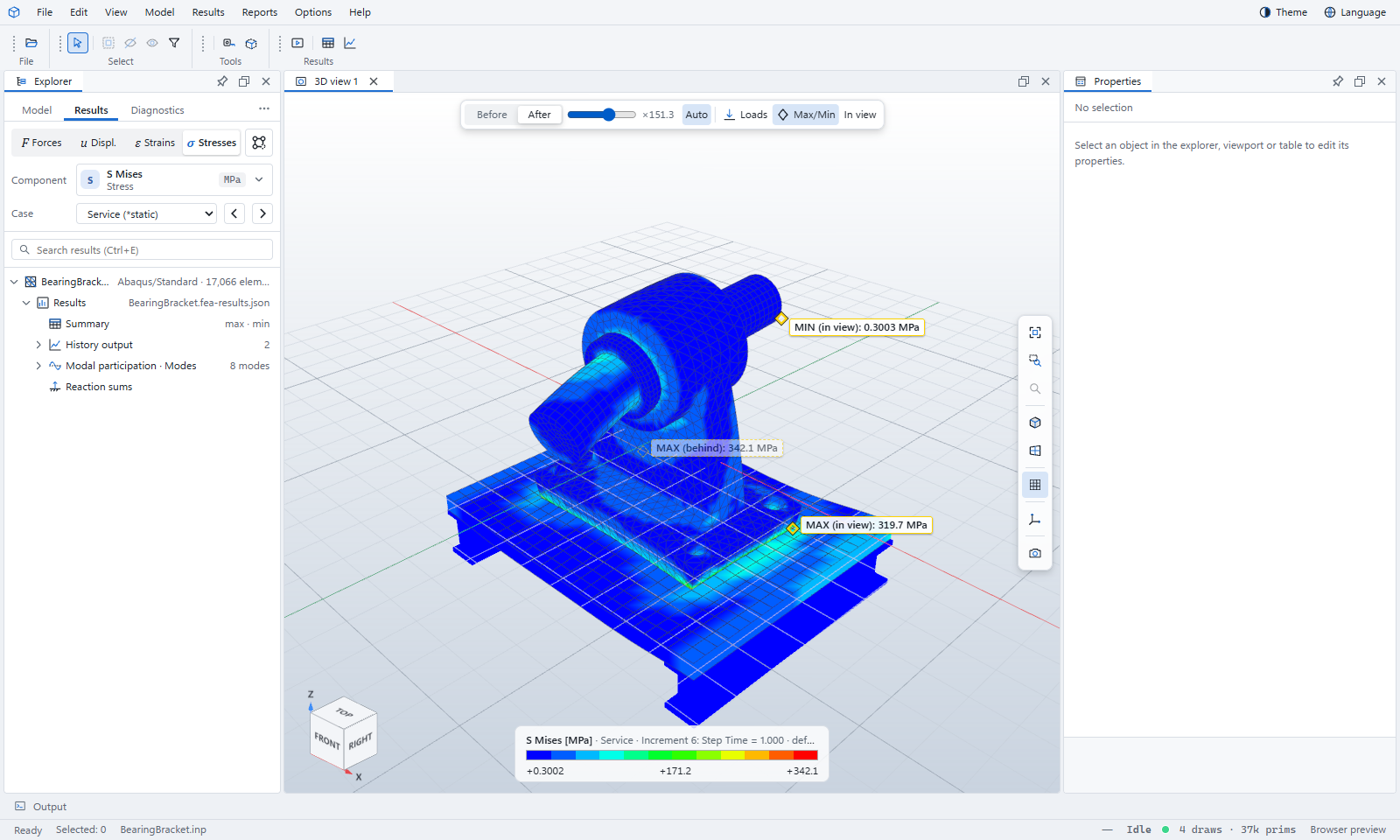
- Open the Results tab and click σ Stresses. The default component is S Mises.
- Open Component to pick another: principal stresses, Tresca, pressure, the six components — every field in the .odb is listed, grouped by family.
- Case lists the steps; the field is shown at the step's last frame.
- Click After to see the deformed shape. The scale is automatic; drag the slider to change it.
4. Frames and animation
Results › Field, frame and deformation sets the frame, where values are taken (integration points, centroids or nodes), the section point of a shell and the coordinate system. Results › Previous and Next step through the frames; Play animates them. A mode shape plays as a smooth back-and-forth swing.
5. Tables and charts
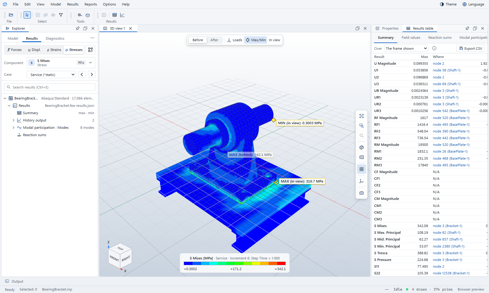
- Reports › Summary table lists the largest and smallest value of every result and the node where it occurs. Click a node to find it in the model; Export CSV saves the table.
- Reports › Reaction sums totals the reactions — a quick check against the applied loads.
- Reports › Modal participation lists the effective mass of each mode, for frequency steps.
- Reports › Charts plots history output, such as energies and reaction forces over time.
6. Job messages
If the job's .msg, .sta and .dat files are beside the results, Reports › Job messages lists their warnings and errors in plain language, with what usually causes them. Reports › Open job messages… reads them from another folder.
Very large jobs
The web Viewer reads .odb files inside your browser, so the size it can manage depends on your computer's memory. For output databases of several gigabytes, use the desktop app: it reads them piece by piece from the disk, and can also export the results with your own Abaqus in one click.